D: 29 Jan 2025

Main functions

  (--make-grm-bin...)

Tutorials

Data Exploration 2 — Genomic Structure

Relationship Matrix

Genome-Wide Assocation Analyses (GWAS)

Post-Hoc

Formatting Files

Variant IDs

Reference Alleles

Format for R

Shortcuts

Quick index search

GWAS 1: Regressions

Significance

The goal of GWAS is to run large genotype-phenotype analyses with the intent of discovering predictive or causal genetic variants using a somewhat hypothesis free approach. That said, the data we use, how it is processed, and selection thresholds can bias results.

Objective

Here we will show the basic operations for running a GWAS analysis for quantitative traits (continuous variables) and qualitative traits (case-control, binary variables).

Since there are no completely public human GWAS datasets, that we know of, we will use a simulated dataset. This was generated by projecting genetic variant effects through the 1000 Genomes Phase 3 (1kGP3) data, thus capturing some real genomic structure across populations.

This was generated using 1kGP3 biallelic, autosomal SNPs; LD-pruned (pairphase 100 0.8); MAF>0.05; HWE P-value>0.05; under the filename all_hg38_qcd_LE1. This was generated in the Linkage tutorial. If you do not have these files under ./data/processed/, then go back to this tutorial or Tutorial Shortcuts - Linkage.

Phenotypes are generated using an ad hoc additive model with genomic effects and Gaussian noise (unexplained variance). Effects are randomly selected with probability k/p, where k are the number of desired non-zero genetic effects and p the total pool of variants to select from (here we used 10,000 random SNPs from the dataset above). Non-zero effects before normalization are 1.

The model is given by:

$y={\sigma }_{a}f(G{u}^T)+{\sigma }_eϵ$

where,
${\sigma }_a$ = standard deviation of the additive genetic effects (akin to narrow-sense heritability, $\sqrt{h^2}$)
$G$ = $n\times p$ genotype matrix with $p$ z-scored genotype columns and $n$ samples
$u^T$ = transpose of the $1\times p$, $u$ genetic effects vector with elements $\in \{0,1\}$
${\sigma }_e$ = standard deviation of the residual error
$ϵ$ = standard normal random variable
$f(x)$ = z-score function

Qualitative traits are further derived by thresholding the Guassian-like y above per the Normal cumulative distribution function to give a prevalence t. This is consistent with the liability-threshold model in genetics. Cases are coded as 2 and controls as 1, which is recognized by Plink 2 and automatically run as a logistic regression.

In the examples below, $h^2\approx 0.9$ with $k\approx 50$ (quantitative trait) or $k\approx 20$ and t=0.1 (qualitative trait).

Before running any of the exercises below, run this file in R.

R:

source("../R/gwas1.R")

Part 1: Quantitative Phenotypes

Here, we'll run some association analyses using a quantitative phenotype. We will use the simulated-gwas simgwas_quant1 in the /GWAS/project1/data/raw/. This is part of the tutorial package.

Plink 2:

time plink2 \ --pfile ./data/processed/all_hg38_qcd_LE1 \ --glm allow-no-covars \ --pheno ./data/raw/simgwas_quant1.pheno \ --pfilter 1e-6 \ --out ./results/gwas/all_hg38_qcd_LE1_simgwas_quant1a --glm allow-no-covars
This runs the generalized linear model (GLM). Plink 2 expects covariates and that omission of this is unintended. Here, we intend to not include covariates and thus use the argument allow-no-covars.

--pheno
Points to the phenotype file.

--pfilter
Here we include a filter on P-values to reduce the size of the glm output files. The value 1e-6 is somewhat arbitrary for these examples.

--out ./results/gwas/all_hg38_qcd_LE1_simgwas_quant1a
Make sure to add the _quant1a tag.

Let's plot the results.

R:

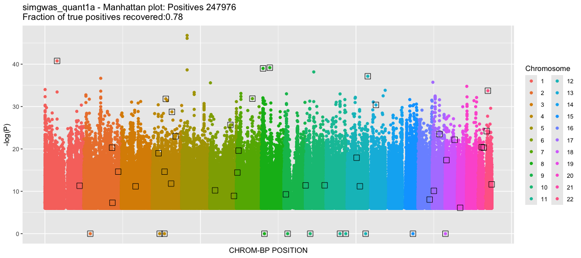
b<-process_gwas_data("simgwas_quant1a","simgwas_quant1","linear")

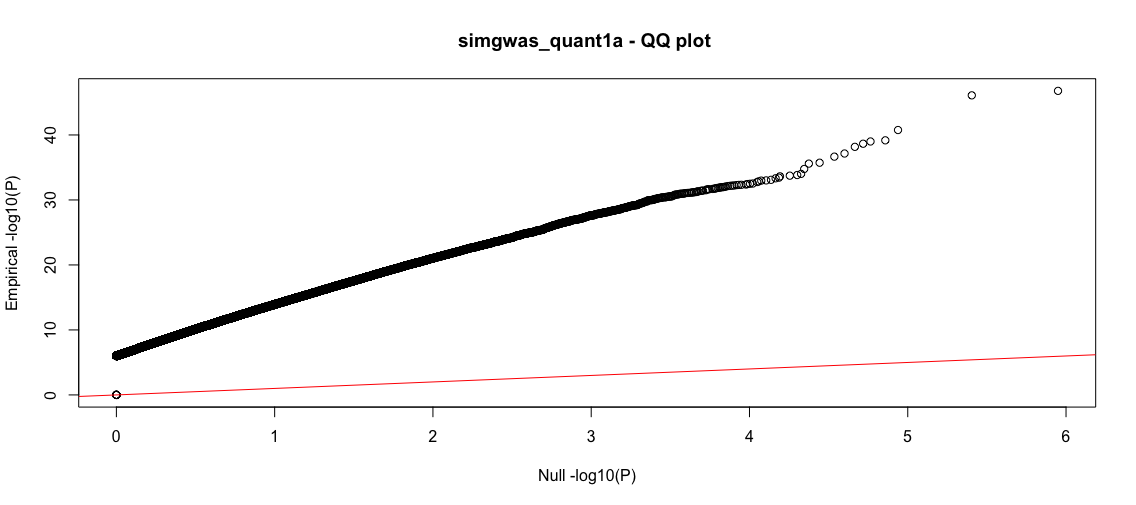
This will produce two plots. For this instance, it will take a few minutes since there are many data points. The first plot is a classic Manhattan plot displaying the -log10(P) values for the SNPs with P-value<1e-6 (the somewhat arbitrary threshold that we set). Following this is a -log10(P) QQ plot, comparing the GLM returned P-value quantiles vs the uniform null.

Wow, so nearly 250K SNPs in the dataset have very small P-values (strong associations). The QQ plot reflects the strong deviation from the null suggesting that these are true effects. As we know the groundtruth, we know that these are in fact many false positives and the true positive rate is far from 1. However, the classic statistical tests are deceptive, suggesting that we have a large yield of true positives. Let's investigate more.

If we think more about the generating model (described above using the 1000 Genomes data), there is a lot of population structure. As you might recall from prior tutorials, part of this structure are varying MAFs across populations even to the point where some minor alleles in one population become major alleles in another. The regression model is identifying not only the trait-causal SNPs but also SNPs that distinguish between populations. Note that we did not explicitly add a population covariate when we simulated the phenotype. Instead, the natural population structure is enough to "distort" the causal signal. This happens because there is a bias in how often true positives occur across different populations. Population identity becomes a significant phenotype signal. We pickup some TPs that are part of that population signal, but also many other SNPs that are only signaling population differences.

Let's test the hypothesis that population structure is the cause of many false positives.

Plink 2:

time plink2 \ --pfile ./data/processed/all_hg38_qcd_LE1 \ --glm hide-covar --covar ./results/qc/qc3/all_hg38_qcd_LE1_pca.eigenvec \ --pheno ./data/raw/simgwas_quant1.pheno \ --pfilter 1e-6 \ --out ./results/gwas/all_hg38_qcd_LE1_simgwas_quant1b

--glm hide-covar --covar ./results/qc/qc3/all_hg38_qcd_LE1_pca.eigenvec
We now add a covariance file, which is our 10 PCs from an earlier tutorial for this dataset. If you don't have this file then run the Relationship Matrix tutorial. The hide-covar is added as to not include the PC-covariate regression coefficients in the glm output file. (They are calculated and used for the regression model, but we aren't interested in their statistics.)

R:

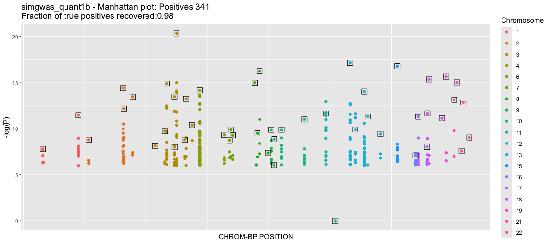
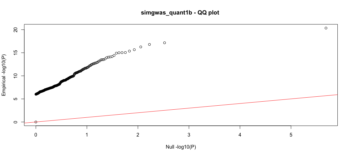
b<-process_gwas_data("simgwas_quant1b","simgwas_quant1","linear")

Good. Now there are about 1000-fold less SNPs that pass the 1e-6 cutoff. We even improve our yeild of known TPs, getting all but one. The QQ plot shows substantial deviation from the null, supporting that these are true effects. We will explore the source of the remaining false positives in another tutorial. We close out this tutorial by showing how to run the qualitative-trait GWAS.

Part 2: Qualitative Phenotype

We have created a GWAS set using the same method above but we thresholded the continuous phenotype to give a case prevalence of 10% (typical case-control are closer to 1% or lower but we have a fairly small sample size, so we are using a higher prevalence). Here we give an example of the commands for running a case-control, logistic model.

Plink 2:

time plink2 \ --pfile ./data/processed/all_hg38_qcd_LE1 \ --glm hide-covar no-firth \ --covar ./results/qc/qc3/all_hg38_qcd_LE1_pca.eigenvec \ --pheno ./data/raw/simgwas_qual1.pheno \ --pfilter 1e-6 \ --out ./results/gwas/all_hg38_qcd_LE1_simgwas_qual1

--glm hide-covar no-firth
This runs the regression model. Plink 2 will automatically detect that the phenotype is case-control when case is coded as 2 and control as 1.
no-firth
By default, Plink 2 uses the penalized logistic regression model by Firth (1993) to deal with the separation problem with logistic regression maximum-likelihood. This can occur with poorly balanced data and small data (including low minor allele counts). See Association Analysis. Without this flag, Plink 2 defaults to a standard logistic regression model and tries Firth if there are issues converging. We suppress it since it's not needed here.

Usage Note: In the console, Plink 2 will note if it is running a logistic model. Also, the output files will have extension *.logistic. If this is not the case, then the linear (quantitative) model was run instead.

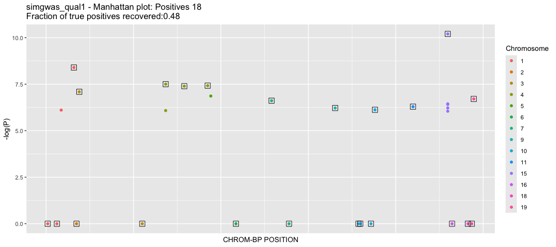
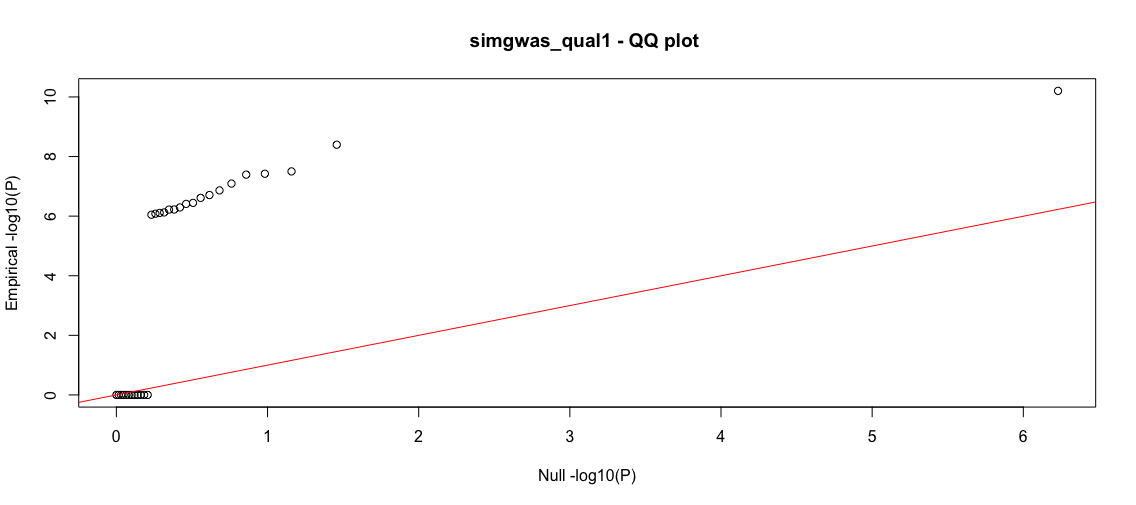
R:

b<-process_gwas_data("simgwas_qual1","simgwas_qual1","logistic")

The yield is not as high as the above quantitative traits; however, we have very low false positives and a sizable return of true positives. As a further exercise, you can try balancing the cases and controls and seeing if that improves discovery.

GWAS 2: Post-Hoc >>