D: 6 Dec 2024

Main functions

  (--make-grm-bin...)

Tutorials

Data Exploration 2 — Genomic Structure

Relationship Matrix

Genome-Wide Assocation Analyses (GWAS)

Post-Hoc

Formatting Files

Variant IDs

Reference Alleles

Format for R

Shortcuts

Quick index search

Data Exploration 2 - Genomic Structure - Relationship Matrix

This is Part B of the Genomic Structure tutorial. If you have not run Linkage, then start there. You can also skip ahead by generating the files from that tutorial, Tutorial Shortcuts - Linkage.

Run this in the R console to load necessary functions for the examples below. If this does not work then make sure you have gone through the Setting Up the Plink 2 Tutorial.

R:

Part 3: Relationships

We start with examining population structure by creating the similarity matrix between individuals (aka relationship matrix), U. Plink 2 has two general methods for this. The first belongs to what is called identity-by-similarity (IBS) and is created using --make-rel (referred here and in Plink as the genomic relationship matrix, GRM). The other belongs to the class of identity-by-descent (IBD) relationship matrices. It is created using --make-king (referred here and in Plink as KING). (Plink 2 uses the KING algorithm from Manichaikul et al., 2010.) The IBS algorithm is agnostic to the genealogical roots between individuals; whereas, IBD methods infer co-segregation of genetic elements from ancestors.

Summary Note: As you will see below, when unaccounted for population structure is a concern, you will want to use KING for relationship filtering.

In practice, KING tends to be more robust to unaccounted for population structure; whereas, such structure distorts GRM estimates. This is not surprising since GRM is essentially a correlation matrix. If the population structure is stronger (accounts for more of the variance) in the sample than familial variance, then the zero-mean and variance normalization will be dominated by this instead of familial relationships. This will distort familial relationship estimates. Let's see these effects and the robustness of KING in practice. Per report, 1kGP3 mostly contains unrelated individuals; however, it also contains some reported parents and their children. We'll generate some relationship matrices and see where unrelated individual pairs and parent-child pairs fall. Make GRM for all individuals in 1kGP3 (about 10 minutes on 2020 M1 MBP).

Plink 2:

time plink2 \ --pfile ./data/processed/all_hg38_qcd \ --make-rel square0 \ --maf 0.1 \ --out ./results/qc/qc3/all_hg38_qcd_grm

--make-rel square0
Makes the GRM relationship matrix as a square matrix with zeros for the upper triangle.

--maf 0.1
Note that previously, we pruned the dataset for maf<0.05. However, Plink 2 may throw an error due to a discrepancy in allele counts in the founder vs nonfounders. Adding a more stringent threshold fixes this. Also, what allele is called minor and the allele counts change with different populations. Thus additional maf pruning may make sense when we isolate subpopulations.

Note: Empirical MAFs are fine down to <sample size>^{-0.5}, i.e. if a MAF estimate of (1/n) is supported by at least n different samples carrying the minor allele, it usually won't be off by enough to matter. So, in the 1kGP3 case this is around 0.02 given ~2,500 founders.

In addition, due to precedence across these tutorials, we used an odd double MAF filtering. (We may change this in future versions of the tutorial.) However, it may make more sense to filter MAFs at the subpopulation level due to substantial cross-population differences and then use the intersection across them to re-pool the subpopulations. Of course, you can only do this if you have some idea of the population structure.

Now, make the equivalent KING matrix (about 5 minutes on 2020 M1 MBP).

Plink 2:

time plink2 \ --pfile ./data/processed/all_hg38_qcd \ --make-king square0 \ --maf 0.1 \ --out ./results/qc/qc3/all_hg38_qcd_king

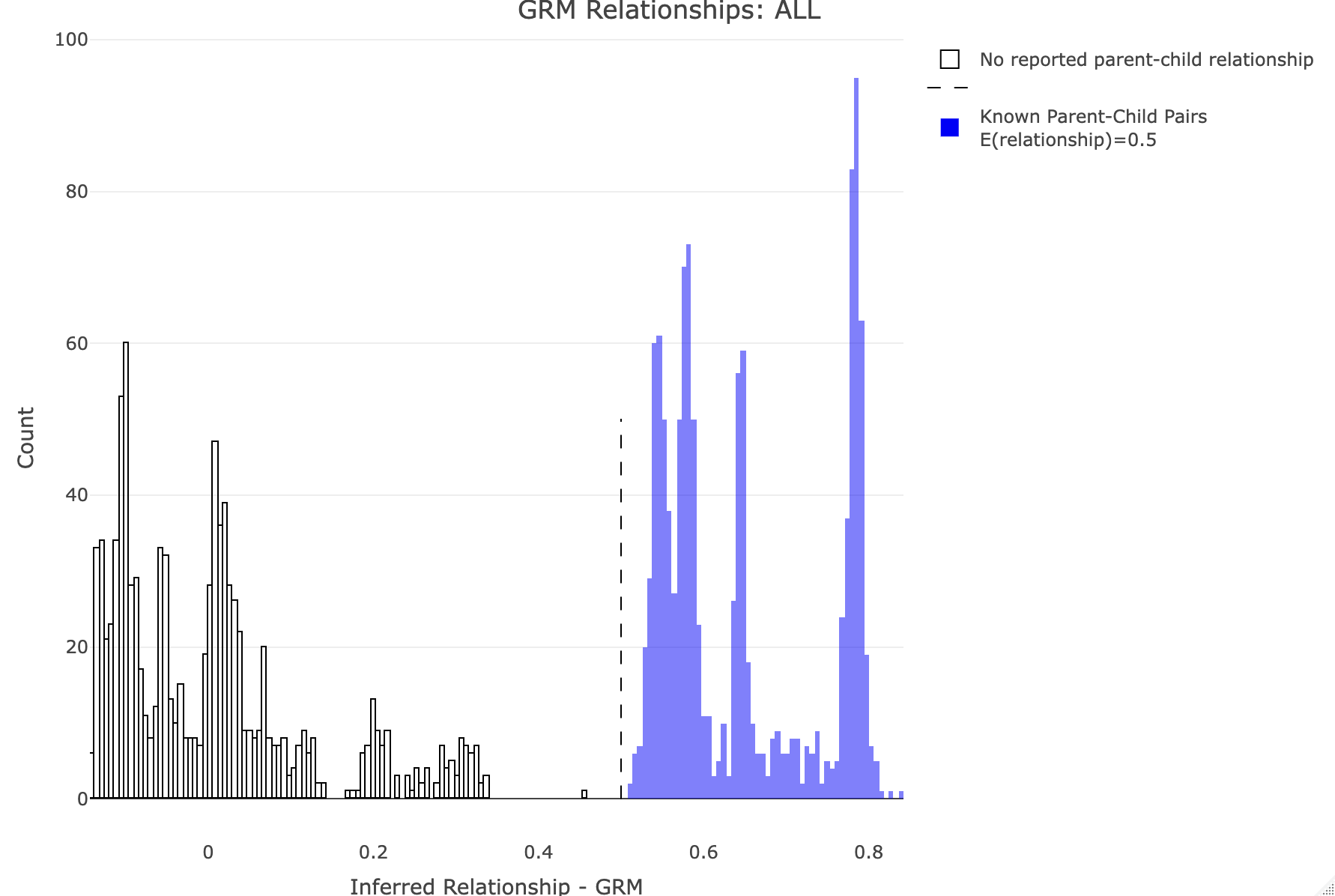
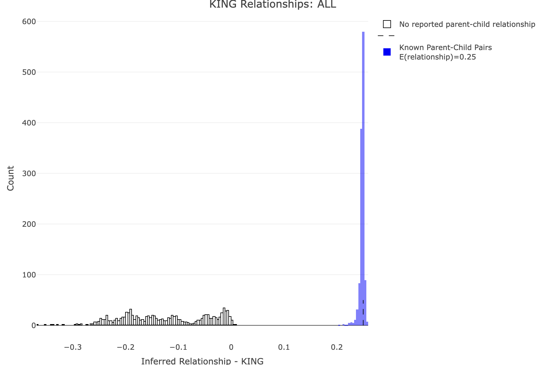
--make-king square0
Makes the KING relationship matrix as a square matrix with zeros for the upper triangle.

Let's plot the distribution of calculated relationships. Note that parent-child pairs are expected to share about 50% of their genomes (for GRM this should be about 0.5, and for KING 0.25). We'll use R to generate some histograms.

R:

Doesn't look great. While there is a clear separation between unrelated and known close relatives (parent-child), the parent-child estimates are much higher than expected and there are apparent strong relationships among reported unrelated individuals. Often, we're interested in filtering-out or -in close relatives. For example, some studies separate unrelated from related using a cutoff of 0.025 for GRM. This will be an issue if those high correlations/relations are artifacts of population structure. You may have also noticed that neither group is unimodal as might be expected for normal-like variation in shared genetics. Okay, let's see what KING says ..

R:

Much better. There is a tight peak around the expected 0.25 for KING. We notice a similar non-Gaussian distribution among unrelated. However, also note that most are estimated to have negative relations. This is not a quirk but a property of the KING algorithm when there is population structure.

Okay, let's play around a bit more. Let's generate GRM and KING matrices for more homogenous populations. Here's example code for selecting the AFR Super Population. Run this for GRM as shown.

Plink 2:

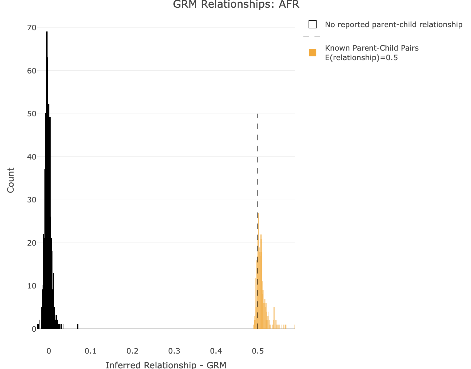
time plink2 \ --pfile ./data/processed/all_hg38_qcd \ --make-rel square0 \ --maf 0.1 \ --keep-if SuperPop==AFR \ --out ./results/qc/qc3/all_hg38_qcd_AFR_grm --keep-if < your rule based on the phenotype data given >
Removes all samples which don't satisfy a comparison predicate on a phenotype or covariate, while --remove-if does the reverse. Syntax and treatment of missing values is the same as for --extract-if-info. For binary phenotypes, either '2' or 'case' (any capitalization) can be used to refer to cases, and either '1', 'ctrl', or 'control' can be used to refer to controls.

In this example, SuperPop is a column label in the all_hg38_qcd.psam file. AFR is a value in that column. SuperPop==AFR is the boolean operator indicating whom to keep. Alternatively, you can use values from a covariate file (see --covar). This command is limited to a single boolean operator.

Plot GRM for AFR

R:

Okay, GRM is performing much better. Close relatives are a bit higher than expected but mostly centered around 0.5. Unrelated are more unimodal. You can run this for KING and see a similar good performance. You can also see if either get better when using an even more homogenous population like the ESN Population (instead of SuperPop, use Population == ESN).

Let's do one more example. Does boiling the cohort down to the country level suffice for other GRM, like AFR apparently did? Run GRM for SuperPop==AMR.

Plink 2:

time plink2 \ --pfile ./data/processed/all_hg38_qcd \ --make-rel square0 \ --maf 0.1 \ --keep-if SuperPop==AMR \ --out ./results/qc/qc3/all_hg38_qcd_AMR_grm

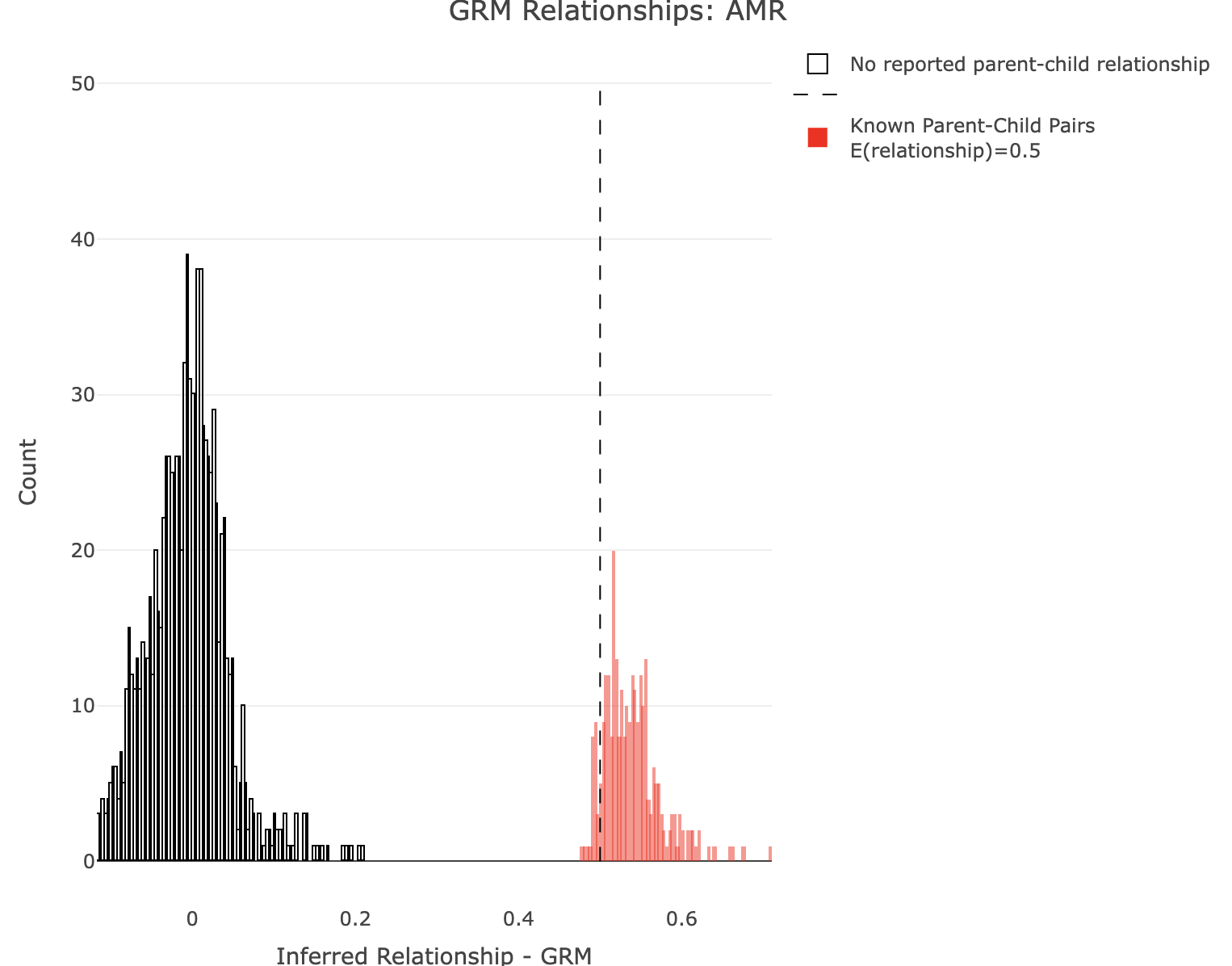
Plot GRM for AMR.

R:

GRM for AMR is almost as bad as for the global dataset.

Let's see how KING does.

Plink 2:

time plink2 \ --pfile ./data/processed/all_hg38_qcd \ --make-king square0 \ --maf 0.1 \ --keep-if SuperPop==AMR \ --out ./results/qc/qc3/all_hg38_qcd_AMR_king

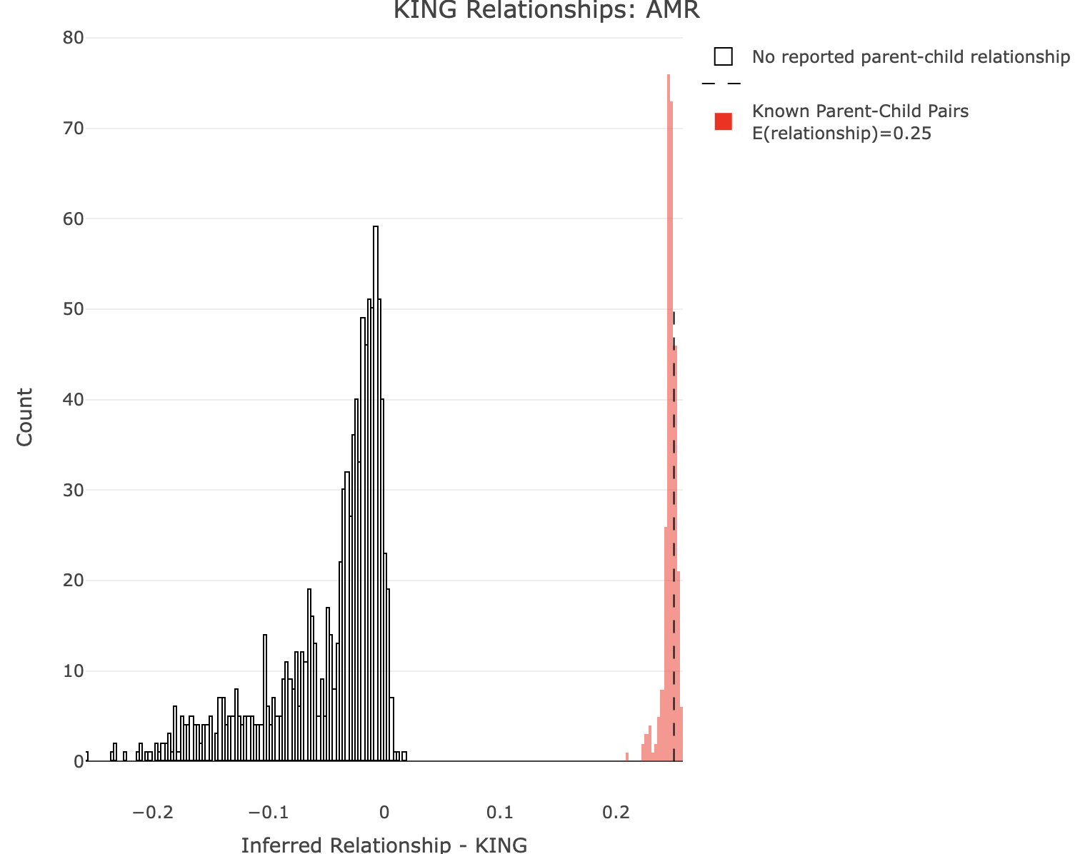
Plot KING for AMR.

R:

Again, KING is robust to this unaccounted for population structure. The KING for AMR infers the correct degree of relation for the parent-child pairs and indicates additional population structure.

We will now take a closer look at population structure.

Part 4. Characterizing Population Structure

Characterizing population structure combines a number of the concepts in the Genomic Structure tutorial set. For this, we leverage the relationship matrix and illustrate how it relates to its dual, the LD or variant space. Population structure is often characterized by decomposing the relationship matrix into principal components or axes of variation, using Principal Components Analysis (PCA). We'll use an LD pruned version of the global population QC'd data. This was generated in the Linkage tutorial. Go back to this tutorial or Tutorial Shortcuts - Linkage, if you do not have these files.

Before we begin, we will remove the 'NA' labelled individuals in 1kGP3.

Create HG-only PCs.

Plink 2:

1. Remove 'NA' individuals

time plink2 \ --pfile ./data/processed/all_hg38_qcd_LE1 \ --make-pgen \ --remove ./misc/naiid.txt \ --out ./data/processed/all_hg38_qcd_LE1_HGonly

--remove ./misc/naiid.txt
Remove all IIDs with 'NA' using the included tutorial file for these ids.

2. Compute HG-only PCs

time plink2 \ --pfile ./data/processed/all_hg38_qcd_LE1_HGonly \ --freq counts \ --keep-founders \ --pca biallelic-var-wts \ --out ./results/qc/qc3/all_hg38_qcd_LE1_HGonly_pca

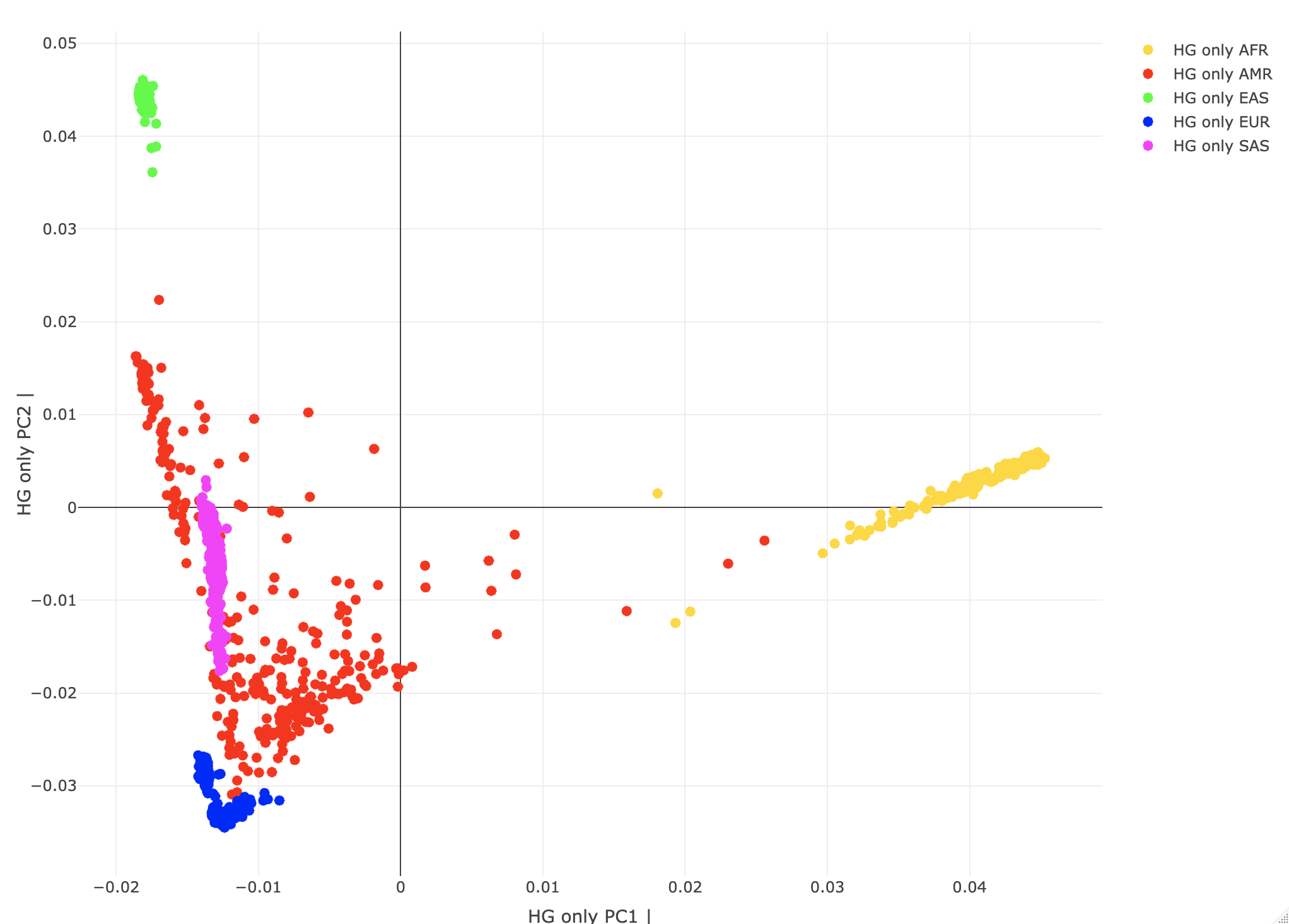
--pca biallelic-var-wts
This runs the PCA on a GRM matrix (computed when calling PCA). The biallelic-var-wts argument saves the allele weights that we will use for projections. We'll talk about this more later.

--freq counts
Generates the allele frequency counts needed for the projections.

Using R, let's plot the HG-only individuals by their "population" PC scores.

A<-gen_popstrat_A('all_hg38_qcd_LE1_HGonly') popstrat_plot2d(A,c("PC1","PC2"), Aprefix="HG only")

Individuals are color-coded by assigned SuperPopulation IDs. (Note R studio plotly is a little quirky with saving/exporting the images. You may need to try exporting it a few times to save.)

We see the population structure that our other analyses were suggesting. Note how AMR is broadly distributed, which explains why the GRM relationships above were so distorted.

Population Projections

Now that we know how to make a population map, let's see how we can project new individuals into this space. That's a nicety of linear algebra. We can perform PCA on people space U and recreate the PCs in the genotype space V, through the SVD identity (underlying PCA) G=UΣV^T. This saves us a lot of unnecessary computation and memory. The people PCs represent loadings across genotypes. So to get PC1 in the genotype space, we take a weighted sum across individual genotypes with weights given by their loading on the people PC1 axis. Fortunately, Plink 2 does this G,U → V mapping for us but with a warning about scaling. Let's see what the scale warning is about by projecting the HG-only data (called REF from here on) through the PCs generated using the exact same HG-only (REF) data. We may hypothesize that these should be exactly the same.

Project REF against the REF-generated allele weights.

Plink 2:

--score <scoring-system vector> #i #j [#k] header-read no-mean-imputation
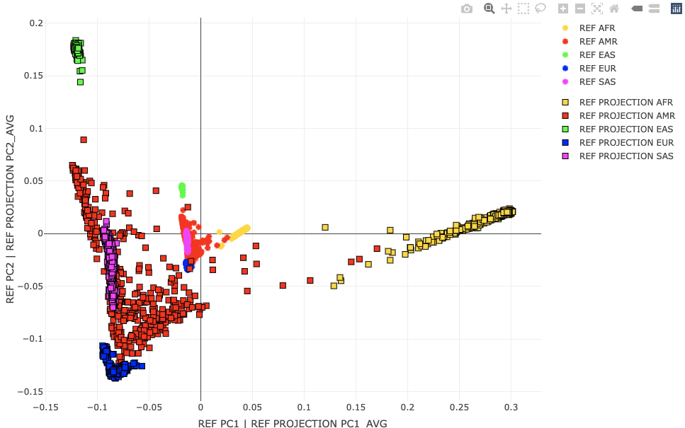
Applies linear scoring system to each sample, and reports results to *.sscore. More precisely, if G is the full genotype/dosage matrix (rows = alleles, columns = samples) and a is a scoring-system vector with one coefficient per allele and then divides by the number of allele observations (i.e. usually twice the number of variants. The input file must have exactly one line per scored allele. Variant IDs are read from column #i and allele codes are read from column j, where i defaults to 1 and j defaults to i+1. 'header-read' causes the first line of the input file to be treated as a header line containing score names. The 'no-mean-imputation' modifier throws out missing observations (decreasing the denominator in the final average when this happens). See Linear scoring, for more details.

--score-col-nums 5-14
By default, a single column of coefficients is read from column #k when using --score, where k defaults to j+1. To specify multiple columns, use --score-col-nums.

--read-freq ./results/qc/qc3/all_hg38_qcd_LE1_HGonly_pca.acount
Loads allele frequency estimates from a --freq (PLINK 1.x ok), --geno-counts, or PLINK 1.9 --freqx report, instead of imputing them from the immediate dataset. This can mitigate issues when a small subset of a larger dataset or population is used.

Now, let's visualize the projected population coordinates for the REF set against their original population coordinates.

R:

The original REF-PC coordinates are relatively the same as the PC-projected REF data but the scale is off.

Take-Home Notes:
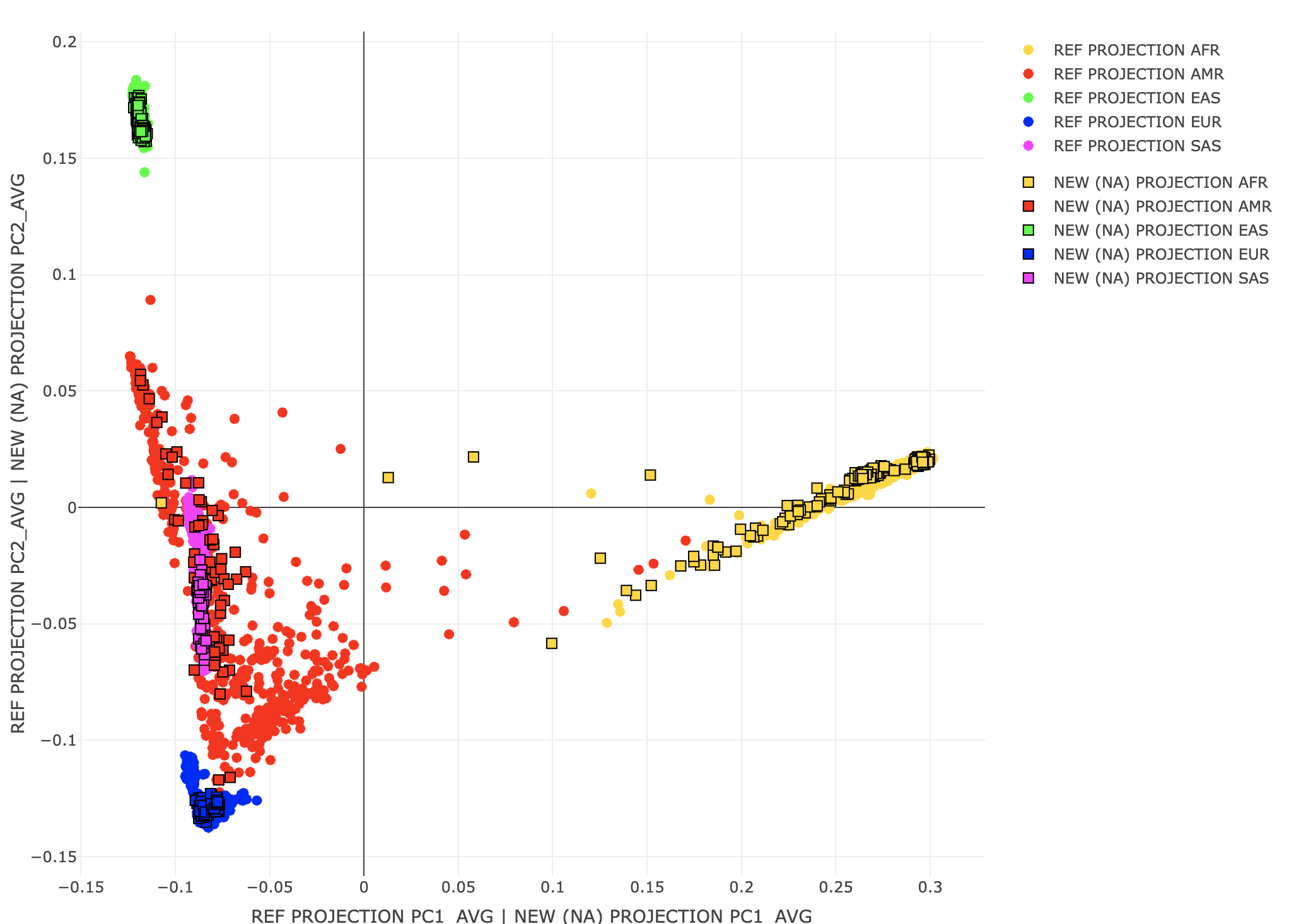
Scaling between the original REF coordinates in the sample PC space and a new sample (or original REF) projected against the variant PCs is challenging. Simply scaling by the singular values does not work. One solution (1) is to use the same projection method for the REF and new samples. However, even this will not always work. One potential issue is underestimating population structure (shrinkage) that can happen with high dimensional problems. A second issue is that these PCs may represent LD structure vs individual differences. In this case, intended population covariates may lower GWAS signal for these genetic variants. Plink 2 may include correction factors in future versions.

For more details we refer you to these references:

• Wang, C., Zhan, X., Liang, L., Abecasis, G. R., & Lin, X. (2015). Improved ancestry estimation for both genotyping and sequencing data using projection procrustes analysis and genotype imputation. The American Journal of Human Genetics, 96(6), 926-937.
• Privé, F., Luu, K., Blum, M. G., McGrath, J. J., & Vilhjálmsson, B. J. (2020). Efficient toolkit implementing best practices for principal component analysis of population genetic data. Bioinformatics, 36(16), 4449-4457.
• Zhang, D., Dey, R., & Lee, S. (2020). Fast and robust ancestry prediction using principal component analysis. Bioinformatics, 36(11), 3439-3446.
• Dey, R., & Lee, S. (2019). Asymptotic properties of principal component analysis and shrinkage-bias adjustment under the generalized spiked population model. Journal of multivariate analysis, 173, 145-164.
• Lee, S., Zou, F., & Wright, F. A. (2010). Convergence and prediction of principal component scores in high-dimensional settings. Annals of statistics, 38(6), 3605.

With the above in mind, let's run a variant of solution (1). We will project new samples and the REF samples and see how those line-up. Thus, both with have some similar scaling. We will project the 'NA' dataset that we removed above before estimating PCs, and see where they project along with the similarily PC-projected REF samples.

Plink 2:

Now using R, plot the projected NA group with the projected REF group.

R:

Beautiful! The new individuals (squares) (not used to create the REF population PCs) line up well with the PC-projected REF samples.

Usage Note: Variations to running PCA projections: For .bed+.bim+.fam datasets or when using --pca allele-wts, add vcols=chrom,ref,alt to the PCA projection recipe (see PCA projection). This allows the recipe to continue working where the output would have an additional PROVISIONAL_REF? column indicating that the REF/ALT alleles are probably just major/minor.

Let's generate the whole 1kGP3 PCs (HG and NA) for later tutorials.

Plink 2:

time plink2 \ --pfile ./data/processed/all_hg38_qcd_LE1 \ --freq counts \ --keep-founders \ --pca biallelic-var-wts \ --out ./results/qc/qc3/all_hg38_qcd_LE1_pca

GWAS 1: Regressions >>