|
D: 11 Mar 2026 Main functions (--make-grm-bin...) Quick index search |
Data Exploration 1 - Basic Statistics (HWE, Allele Frequency Spectrum)SignificanceThere are a set of basic statistics that are useful to investigate prior to running genome analyses. These serve several important purposes including evaluating for: 1) genotyping errors and finite sampling effects, and 2) deviations from assumed genetic models.ObjectiveIn this tutorial we will experiment with two common statistics:Hardy-Weinberg Equilibrium (HWE) and the Allele Frequency Spectrum We will explore these statistics in this tutorial. The major take home point is to account for population structure before filtering on these statistics. There are several approaches when the structure is known or unknown but suspected. For HWE, see the --hwe reference and the keep-fewhet modifier. In the exercises below, we will illustrate how to check if this will be useful and why this can help. However, this does not address population biases that can occur with minor allele frequency (MAF) filtering. Alternatively when population structure is known or inferred as we illustrate in other tutorials, it may make sense to filter genetic variants on HWE and MAF at the subpopulation level and then use the intersection across them to re-pool the subpopulations. Finally, also see Plink 2 Rules of Thumb about MAF filtering. Set the terminal directory to the /GWAS/project1/ using cd commands. All exercises below expect that these steps have been done. setwd("<your path to GWAS>/GWAS/project1/")
source("../R/loadplink2HW.R")
Part 1: Testing for Hardy-Weinberg Equilibrium (HWE)Testing HWE is important for evaluating genotype errors and population structure. Plink 2 uses the Exact-test approach, which conditions for sample size. See Graffelman for more details about the Exact-test and --hardy reference material for different P-value options in Plink 2. Run this to calculate some HWE stats. Plink 2:time plink2 \
--pfile 'vzs' ./data/raw/all_hg38 \
--hardy \
--snps-only \
--autosome \
--keep-founders \
--thin-indiv-count 100 \
--thin-count 100000 \
--seed 111 --threads 1 --memory 8000 require \
--out ./results/qc/qc1/all_hg38_HW_ALLPOP
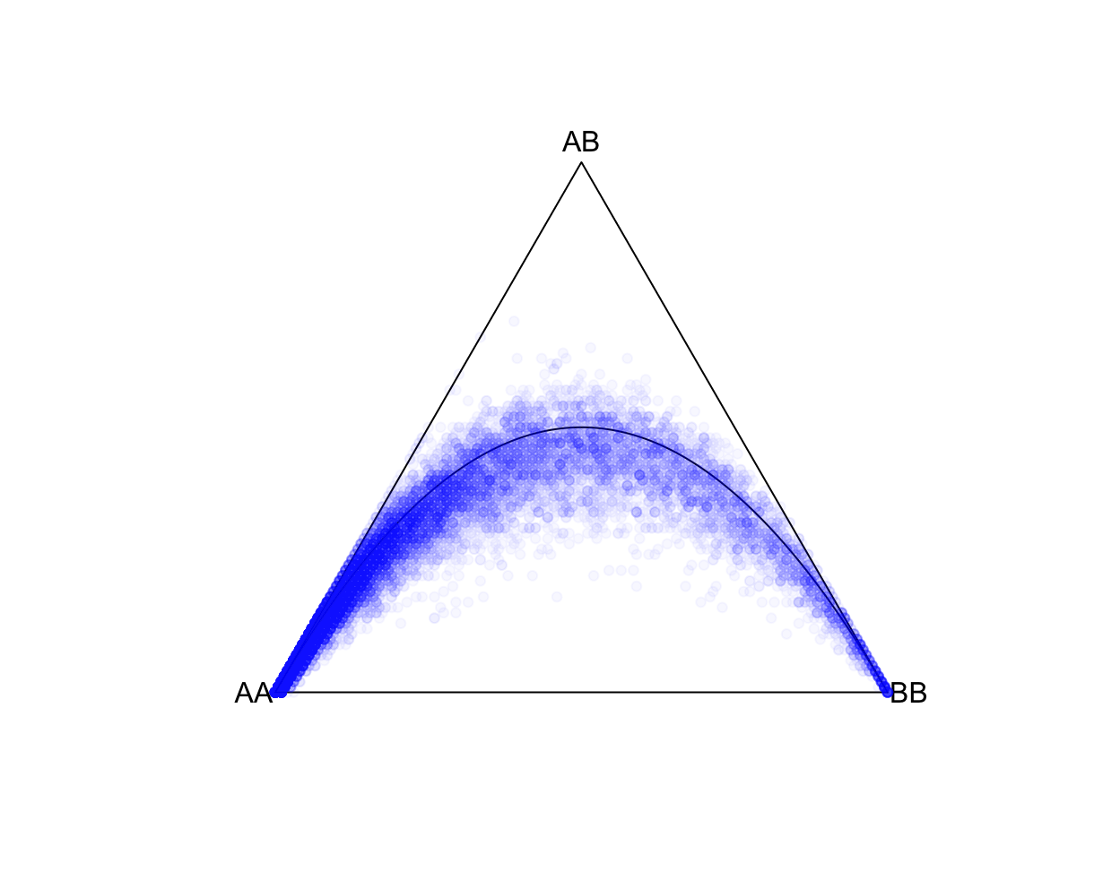
--pfile 'vzs'The set of genotype files to use in the Plink 2 genotype file format. The 'vzs' modifier tells PLINK to look for the extension *.pvar.zst instead of a *.pvar file. --hardy Writes autosomal Hardy-Weinberg equilibrium Exact-test statistics to <output filename>.hardy[.zst], and/or chrX test statistics to <output filename>.hardy.x[.zst]. In this case, it will not write the *.hardy.x file as we are restricting to autosomes. Excludes all variants with one or more multi-character allele codes. With 'just-acgt', variants with single-character allele codes outside of {'A', 'C', 'G', 'T', 'a', 'c', 'g', 't', <missing code>} are also excluded. --autosome Excludes all unplaced and non-autosomal variants. --keep-founders Excludes all samples with at least one known parental ID (non-founders) from the current analysis (note that it is not necessary for that parent to be in the current dataset). We will only keep 100 founders. This is because we will compare the "global" population statistics estimated here against subpopulations in 1000 Genomes, which only have ~100 founders. For this, we use --keep-founders and --thin-indiv-count of 100. --thin-indiv-count n Removes samples (e.g., individuals) at random until only n remain. We will only keep 100 founders. This is because we will compare the "global" population statistics estimated here against subpopulations in 1000 Genomes, which only have ~100 founders. For this, we use --keep-founders and --thin-indiv-count of 100. --thin-count n Removes variants at random until only n remain. --seed 111 --threads 1 --memory 8000 require Parameters for random sampling to ensure that the same random samples are selected. --out <output filename prefix> After running successfully, two files will be generated in the ./results/qc/qc1/ folder: all_hg38_HW_ALLPOP.hardy and all_hg38_HW_ALLPOP.log. Let's explore all_hg38_HW_allpop.hardy. We will make a ternary plot. This projects each SNP onto a three axis grid, where the proximity of the SNP location to a vertex represents the relative proportion of that component. For example, a SNP located at the AA vertex means that AA is the only genotype. A SNP located in the middle means equal proportions of AA, AB, and BB. Also shown, is the theoretical HWE curve. R: fname = "./results/qc/qc1/all_hg38_HW_ALLPOP.hardy"
data<-loadplink2Rmat(fname)
HWTernaryPlot(data[,5:7],region=0,markercol = rgb(0,0,1,0.03),vertexlab = c("AA","AB","BB"))
time plink2 \
--pfile 'vzs' ./data/raw/all_hg38 \
--hardy \
--snps-only \
--keep-if Population==JPT \
--autosome \
--thin-count 100000 \
--seed 111 --threads 1 --memory 8000 require \
--out ./results/qc/qc1/all_hg38_HW_JPT
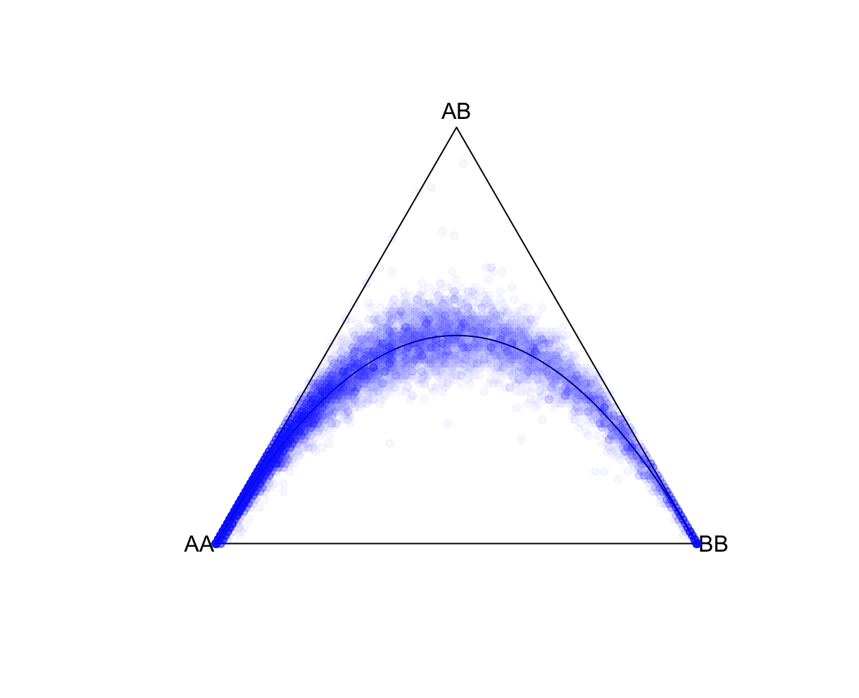
--keep-if <your rule based on the phenotype data given>Removes all samples which don't satisfy a comparison predicate on a phenotype or covariate, while --remove-if does the reverse. Syntax and treatment of missing values is the same as for --extract-if-info. For binary phenotypes, either '2' or 'case' (any capitalization) can be used to refer to cases, and either '1', 'ctrl', or 'control' can be used to refer to controls. In this example, Population is a column label in the all_hg38.psam file. JPT is a value in that column. Population==JPT is the boolean operator indicating whom to keep. This command is limited to a single operator like this one. Alternatively, you can use values from a covariate file (see --covar). R: fname = "./results/qc/qc1/all_hg38_HW_JPT.hardy"
data<-loadplink2Rmat(fname)
HWTernaryPlot(data[,5:7],region=0,markercol = rgb(0,0,1,0.03),vertexlab = c("AA","AB","BB"))
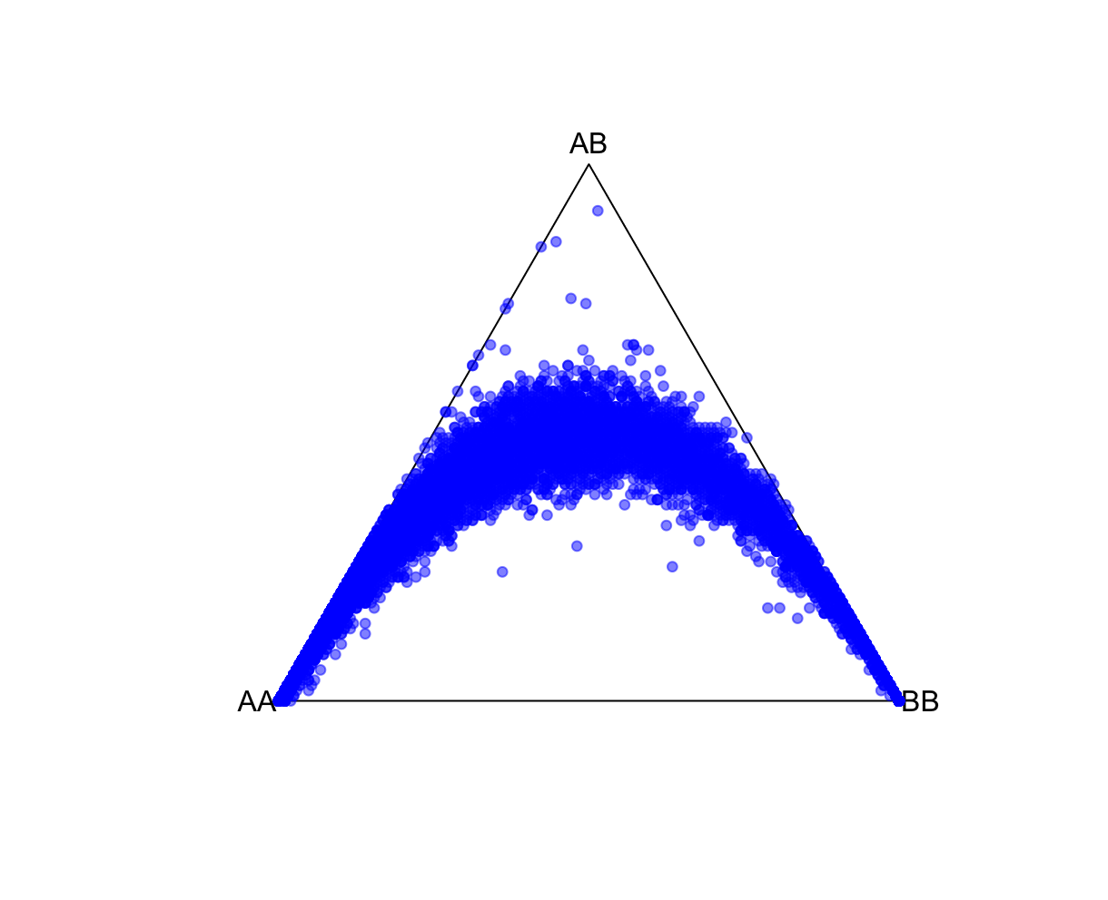
HWTernaryPlot(data[,5:7],region=0,markercol = rgb(0,0,1,0.5),vertexlab = c("AA","AB","BB"))
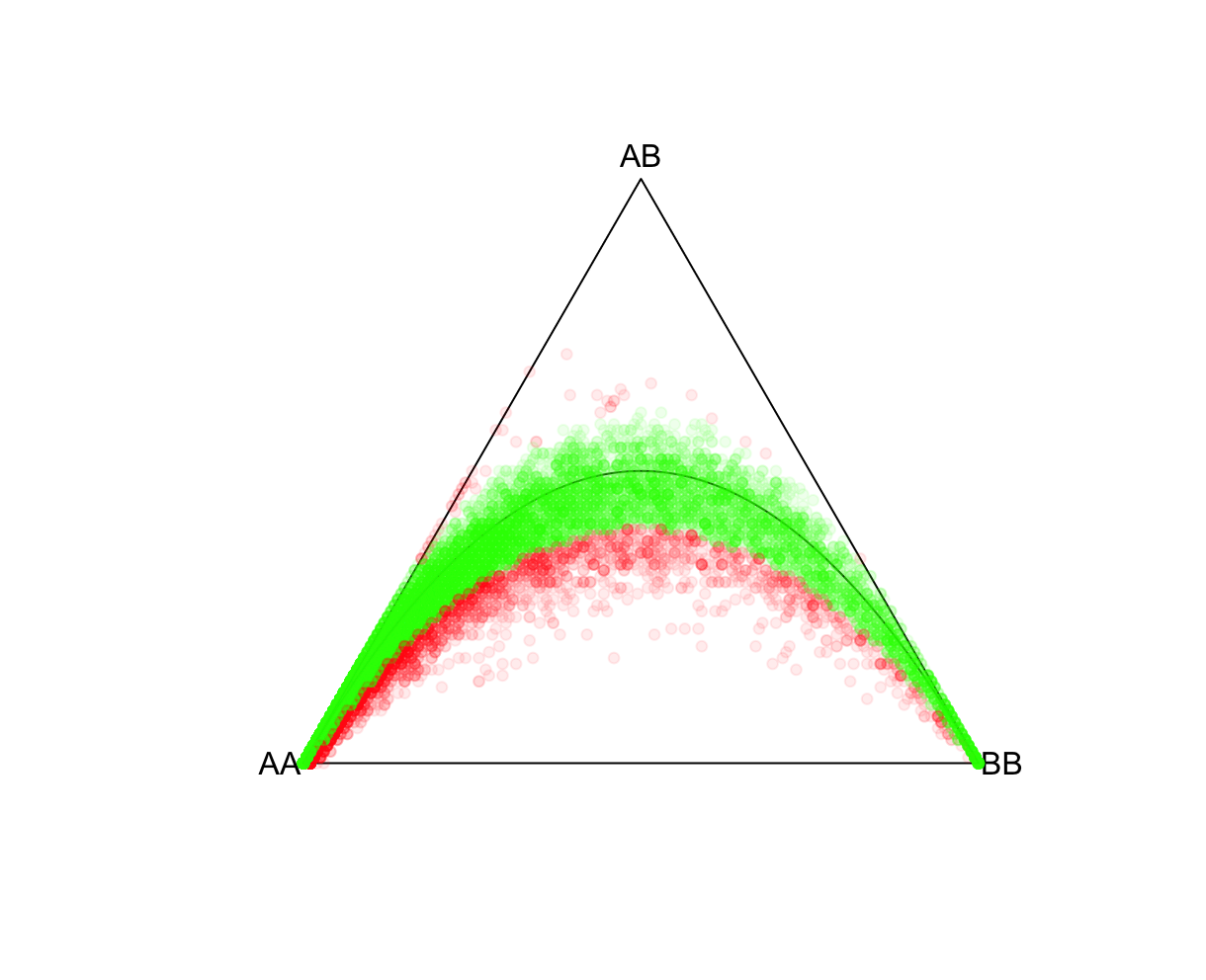
P-value cutoffsSelecting an appropriate P-value threshold is an important component of preprocessing. However, accounting for population structure should be done prior to such thresholding. As expected from the above exercise, ignoring population structure may result in many variants unnecessarily being removed. Reload the ALLPOP HW results and now let's tag all SNPs with a Plink 2 Exact-test estimated P-value<0.05. Side note, the R function pvcut2rgba() uses a default P-value cutoff of 0.05 (alpha refers to R's transparency parameter, not the P-value). R:fname = "./results/qc/qc1/all_hg38_HW_ALLPOP.hardy"
data<-loadplink2Rmat(fname)
mcolor = pvcut2rgba(data,alpha=0.08)
HWTernaryPlot(data[,5:7],region=0,vertexlab = c("AA","AB","BB"),markercol=mcolor)
fname = "./results/qc/qc1/all_hg38_HW_JPT.hardy"
data<-loadplink2Rmat(fname)
mcolor = pvcut2rgba(data,alpha=0.08)
HWTernaryPlot(data[,5:7],region=0,vertexlab = c("AA","AB","BB"),markercol=mcolor)
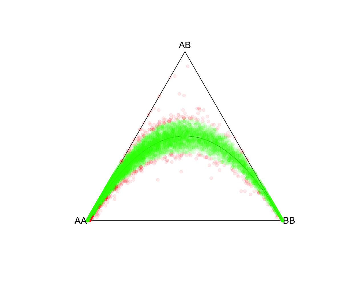
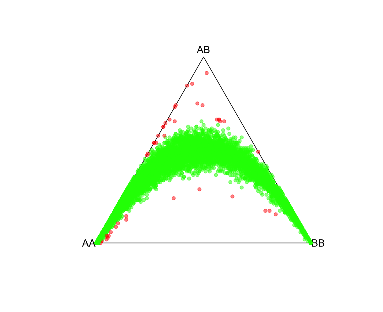
fname = "./results/qc/qc1/all_hg38_HW_JPT.hardy"
data<-loadplink2Rmat(fname)
mcolor = pvcut2rgba(data,pvcut=1e-3,alpha=0.8)
HWTernaryPlot(data[,5:7],region=0,vertexlab = c("AA","AB","BB"),markercol=mcolor)
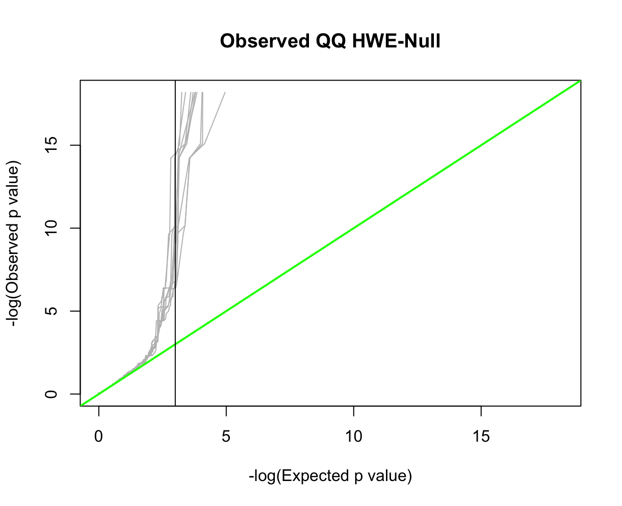
QQ-plotsFor this, we'll use HardyWeinberg package function HWQqplot() (see package link for details). This will plot the Plink 2 observed P-values using the Exact-test versus that expected using the Levene-Haldane probability distribution. HWQqplot() takes about 2 minutes for nsim=10 on a 2020 M1 Macbook Pro. R:fname = "./results/qc/qc1/all_hg38_HW_JPT.hardy"
data<-loadplink2Rmat(fname)
data2 <- format_hwdata2hwpack(data)
HWQqplot(data2,nsim=10,logplot=TRUE, main="Observed QQ HWE-Null")
abline(v=3,color='black',lty=1)
Part 2: Allele Frequency SpectrumAnother common step in GWAS preprocessing is pruning for minor allele frequency (MAF) (e.g., selecting for common variants, MAF>0.05). There are number of reasons why MAF filtering is done. We won't go into detail here. However, when pruning on MAF it is useful to note that allele frequencies are not constant across subpopulations; the major and minor alleles can even switch (see rs3115858 in dbSNP, for example). In this exercise, we'll explore how the allele frequency changes across subpopulations. First, let's look get the allele spectrum for the ALLPOP (global) pool. We'll use Plink 2's --freq with flag alt1bins=. Plink 2:time plink2 \
--pfile 'vzs' ./data/raw/all_hg38 \
--freq alt1bins=0.01,0.02,0.03,0.04,\
0.05,0.06,0.07,0.08,0.09,0.10,0.11,0.12,\
0.13,0.14,0.15,0.16,0.17,0.18,0.19,0.20,\
0.21,0.22,0.23,0.24,0.25,0.26,0.27,0.28,\
0.29,0.30,0.31,0.32,0.33,0.34,0.35,0.36,\
0.37,0.38,0.39,0.40,0.41,0.42,0.43,0.44,\
0.45,0.46,0.47,0.48,0.49,0.50,0.51,0.52,\
0.53,0.54,0.55,0.56,0.57,0.58,0.59,0.60,\
0.61,0.62,0.63,0.64,0.65,0.66,0.67,0.68,\
0.69,0.70,0.71,0.72,0.73,0.74,0.75,0.76,\
0.77,0.78,0.79,0.80,0.81,0.82,0.83,0.84,\
0.85,0.86,0.87,0.88,0.89,0.90,0.91,0.92,\
0.93,0.94,0.95,0.96,0.97,0.98,0.99,1.00 \
--snps-only \
--autosome \
--keep-founders \
--thin-count 100000 \
--seed 111 --threads 1 --memory 8000 require \
--out ./results/qc/qc1/all_hg38_freq_ALLPOP_keepall
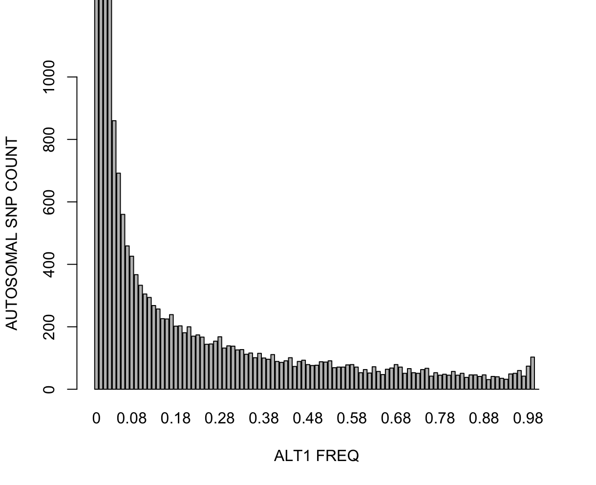
Main command that calculates the ALT allele frequencies (there is counterpart for REF as well) and bin-counts the variants within the given frequency edges. This will output a histogram file with extension *.afreq.alt1.bins. Let's plot this in R. R: fname = "all_hg38_freq_ALLPOP_keepall.afreq.alt1.bins"
data = loadplink2Rmat(paste0('./results/qc/qc1/', fname))
barplot(unlist(data['OBS_CT']),names.arg=unlist(data['BIN_START']),ylim=c(0,1000),xlab="ALT1 FREQ",ylab="AUTOSOMAL SNP COUNT")
time subpops=("LWK" "ASW" "CHB" "JPT")  \

for subpop in "${subpops[@]}"; do
plink2 --pfile 'vzs' ./data/raw/all_hg38 \
--freq \
--snps-only \
--autosome \
--keep-founders \
--thin-count 100000 \
--seed 111 --threads 1 --memory 8000 require \
--keep-if 'Population=='$subpop'' \
--out ./results/qc/qc1/all_hg38_FREQ_$subpop
done
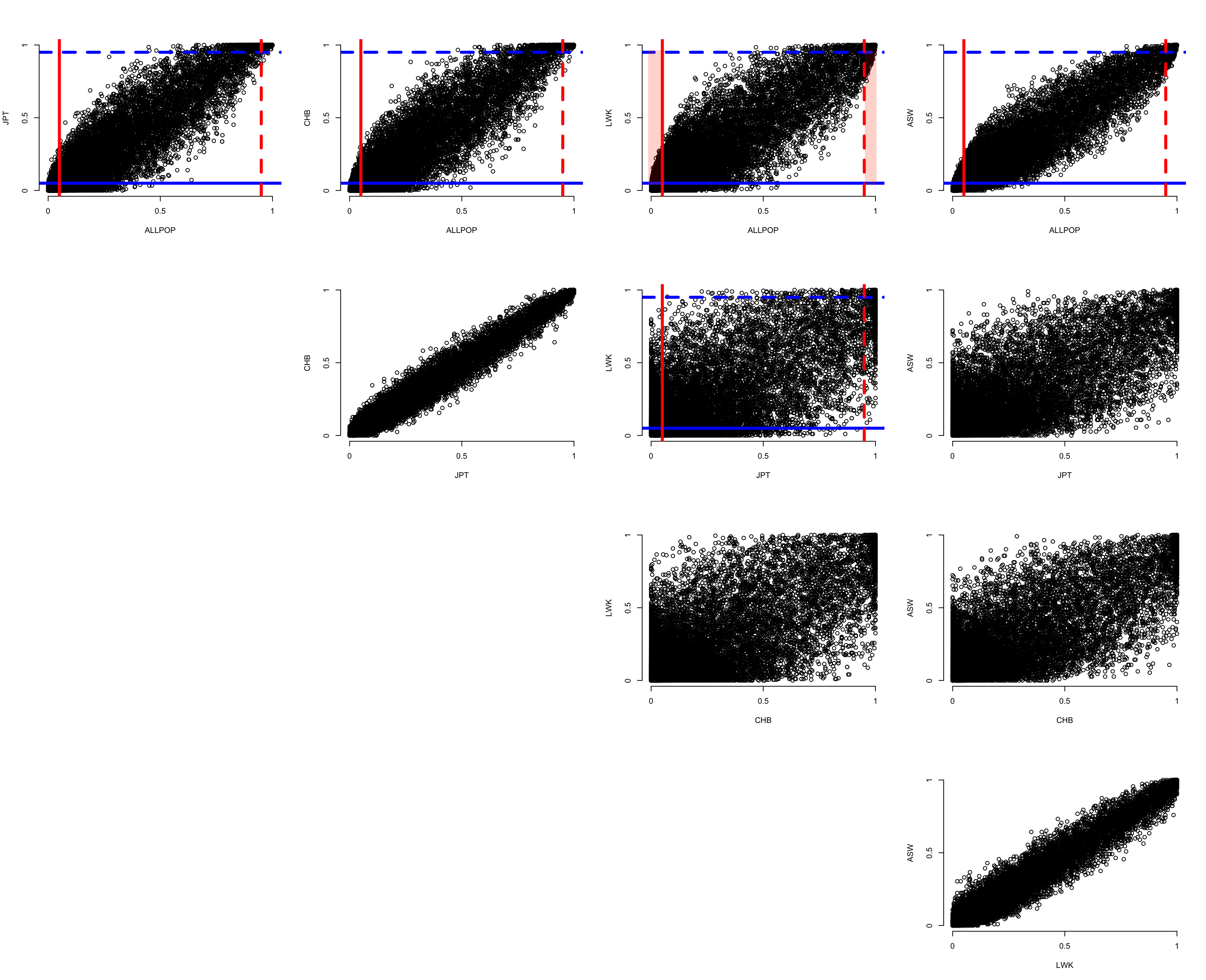
Shell command that loops through the Population labels, estimating the REF and ALT allele frequencies using --freq. We will compare the ALT frequencies across Populations.
Once these are generated, then in R: source("../R/AScompare.R")
This will generate a plot similar to below (without the red shaded areas). Give it a minute or so to process, and use Zoom after the plot is rendered.
source("../R/HWvsFREQ.R")
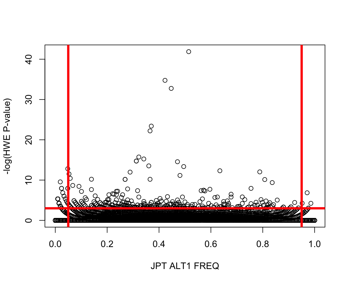
|